R Project - Calculating VaR of FTSE100 time series data using GARCH models.

Quick Summary

In this project we shall investigate the use of GARCH models for calculating Value at Risk (VaR). Specifically we will fit a GARCH(1,1) model to a time-series data set of FTSE100 closing prices between 7 November 2002 and 6 October 2010 before comparing our results with previous results attained using other methods for calculating VaR. We will discuss the appropriateness of the GARCH model assumptions for our data setand look at fitting other GARCH models to attain improved VaR predictions. Finally, we will discuss our results in terms of the literature on modelling volatility using GARCH models.

1   Introduction

We aim to investigate the appropriateness of the GARCH model for modelling FTSE100 closing prices. We will fit the proposed model to the 1000 most recent log returns from the FTSE100 data set before evaluating whether the data is conditionally normal by performing a Q-Q plot. We will then be able to predict the Value at Risk for a period of 24 hours for £1000 invested in a FTSE Index Fund and then use cross-validation to evaluate this approach. In our discussion we will compare our result with previous workshop results as well as considering the appropriateness of the GARCH model assumptions for the FTSE100 data. We will conclude by looking to fit other GARCH models as well as considering our results in terms of the literature on modelling volatility using GARCH models.

We conduct our analysis using the programming language r. We begin by first importing the rugarch, tseries, ggplot2, reshape, gridExtra and kableExtra package libraries.

 1
 2
 3
 4
 5
 6
 7
 8
 9
10
11

## Import libraries
library(rugarch)
library(tseries)
library(ggplot2)
library(reshape)
library(gridExtra)
library(kableExtra)
library(ggdark)
## import data
source("FTSE.R")
options(knitr.table.format = "html") 

2   Model Fitting

We consider a data set containing the daily returns from the FTSE100 from 7 November 2002 to 6 October 2010. We produce the time series plot of this data, shown below in Figure 1 below.

 1
 2
 3
 4
 5
 6
 7
 8
 9
10
11
12

FTSE=FTSE.close
time = 1:length(FTSE)

n=length(FTSE)
X=log(FTSE[(n+1-1000):n]/FTSE[(n-1000):(n-1)])

# Produce plot for figure 1
fig1 = data.frame(time, FTSE)
plot1 = ggplot(data = fig1, aes(time,FTSE))+geom_line(col=2) + 
  ggtitle("FTSE100 Time Series Data from 07-11-2002 to 06-10-2010.") +
  xlab("Time (t)") + ylab("Closing Price")
plot1

We fit the following model to the 1000 most recent log returns from the FTSE100 data set:

\[X_t=\mu+Y_t,\]

where $Y_t$ is a $\text{GARCH}(1,1)$ model with:

\[Y_t\sim\sigma_t, ~~~~\epsilon\sim \text{N}(0,1)\] \[\sigma^2=\omega+\alpha_1\ Y_{t-1}^2+\beta_1\sigma_{t-1}^2\]

To estimate $\mu$ we will use the sample (empirical) mean of the 1000 most recent log returns. The Q-Q plot of the residuals generated from this model is shown below in Figure 2.

 1
 2
 3
 4
 5
 6
 7
 8
 9
10
11

## Last 1000 log returns
mu=mean(X)
Y=X-mu

# Fitting GARCH(1,1) Model
out.garch11=garch(Y, order=c(1,1))

## Computing Residuals & QQ Plot 
res=Y/out.garch11$fitted[,1]
qqnorm(res)
qqline(res)

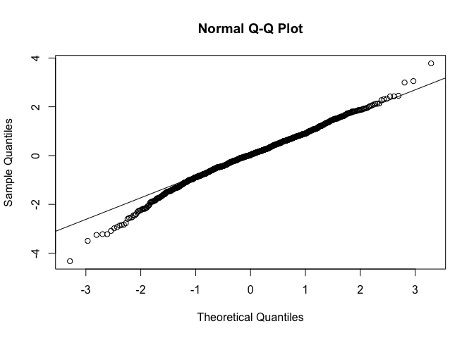
We can see that the data appears to be left-skewed which is an indication that the data is not conditionally normal given $\sigma_t$.

By using this $\text{GARCH}(1,1)$ model we can predict the Value-at-Risk (VaR) for both $\alpha=0.1$ and $\alpha=0.01$ for a period of 24-hours for £1000 invested in a FTSE100 index fund.

1
2
3
4
5
6
7
8
9

## Estimate of sigma^2 for next obs
sigsq=out.garch11$coef[1]+out.garch11$coef[2]*Y[1000]^2+out.garch11$coef[3]*out.garch11$fitted[1000,1]^2

## Calculating VaR
alpha=c(0.1,0.01)
calpha=qnorm(alpha) ##alpha quantile
VaR=1000*(1-exp(mu+calpha*sqrt(sigsq)))
VaR
## [1] 11.71906 21.10751

In summary, for this model we obtain the following values for the VaR:

\[\text{VaR}_{(\alpha=0.1)}=£11.72,\]

\[\text{VaR}_{(\alpha=0.01)}=£21.11.\]

Next we use cross-validation to evaluate this approach for estimating VaR.

 1
 2
 3
 4
 5
 6
 7
 8
 9
10
11
12
13
14
15
16
17
18
19
20
21
22

Xfull=log(FTSE[2:n]/FTSE[1:(n-1)])

N=length(Xfull)
m=1000
I=rep(0,1000)
alpha=0.01

for(i in 1:(N-m)){
  Xrnew=Xfull[i:(m+i-1)] ##data to use at step i of CV
  mu=mean(Xrnew)
  Ynew=Xrnew-mu
  out.garch21=garch(Ynew,order=c(2,1))
  sigsq=out.garch21$coef[1]+out.garch21$coef[2]*Ynew[m]^2+out.garch21$coef[3]*out.garch21$fitted[m,1]^2
  
  
  calpha=qnorm(alpha) ##alpha quantile
  VaR=1000*(1-exp(mu+calpha*sqrt(sigsq)))
  
  I[i]=(1000*(1-exp(Xfull[m+i]))>VaR)
}
sum(I)/(N-m)
## [1] 0.05105105

Therefore, we find that for $\alpha=0.1$, the loss exceeds the VaR about 5.1% of the time.

3   Comparison

In this section I will be using results obtained in my university workshops in which I considered several different ways of estimating the VaR for the FTSE100 data set in consideration. The results of these workshops is details in Table 1 below.

The normal, non-parametric and Laplacian estimates for the VaR were all calculated assuming that the distribution of all log-returns that we have observed is the same. This may be a poor assumption as we have some data which is decades old and so we consider these estimates to be inferior. Additionally, for the three stochastic models we considered we used cross-validation to evaluate their approach to estimating VaR. The results of our investigation are shown in Table 2 below.

If our chosen model fits well then the loss will exceed the VaR less often and so we can see that the $\text{GARCH}(1,1)$ model is the best fit so far for both $\alpha=0.1$ and $\alpha=0.01$.

4   Model Evaluation

We create a plot of the log-returns of the FTSE100 return series over time, shown below in Figure 3.

 1
 2
 3
 4
 5
 6
 7
 8
 9
10
11

FTSE1=diff(log(FTSE.close))
time1 = 1:(length(FTSE)-1)

n=length(FTSE1)

# Produce plot for figure 3
fig3 = data.frame(time1, log(FTSE1))
plot3 = ggplot(data = fig3, aes(time1,FTSE1))+geom_line(col=2) + 
  ggtitle("FTSE100 Log-Returns Time Series Data from 07-11-2002 to 06-10-2010.") +
  xlab("Time (t)") + ylab("Log Returns")
plot3

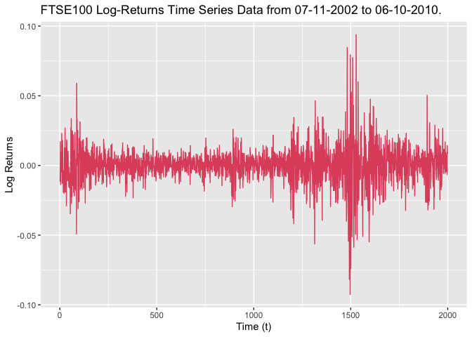
From this plot we can see that the data appears to have a mean of 0 and that there are clear signs of volatility clustering. This suggests that the use of the GARCH model is appropriate. However, the GARCH model we are currently using also makes the assumption that the residuals of the model are normally distributed and our Q-Q plot in Figure 2 would suggest this is not the case. It would make more sense to git a GARCH model which instead assumes the residuals follow a left-skewed, heavy tailed distribution.

5   Other GARCH Models

So far we have considered an $\text{ARCH(1)}$ model, a Laplacian $\text{ARCH}(1)$ model and a $\text{GARCH}(1,1)$ model. Our results suggest that the $\text{GARCH}(1,1)$ model produced the most reliable estimate for the VaR and we consider how we could further improve on this model. We conduct the same analysis for the $\text{ARCH}(5)$ model and the $\text{GARCH}(2,1)$ and show the results of our cross-validation in Table 3 below.

None of the models considered above have improved upon our initial $\text{GARCH}(1,1)$, therefore any significant further improvements on the model will most likely arise from considering asymmetric variations of the GARCH model such as the Exponential GARCH (EGARCH) model.

6   Discussion

The Q-Q plot for our $\text{GARCH}(1,1)$ model is negatively skewed. This could be evidence of the asymmetric information phenomenon in the fluctuations of financial time series - namely the fluctuations caused by bad news are always much greater than those of good news. This phenomenon has been the topic of a large amount of academic literature, including articles by Black(1976), French(1987), Nelson(1990) and Zakoian(1994).

There have been numerous studies investigating the utility of EGARCH and GJR-GARCH models when it comes to modelling of stock market volatility. For example, @Danielson1994 found in estimating the daily S&P500 Index data from 1980 to 1987 that the $\text{EGARCH}(2,1)$ model outperformed the $\text{ARCH}(5)$, $\text{GARCH}(1,2)$ and $\text{IGARCH}(1,1,0)$. Additionally a study by Najand(2003) attempted to forecast stock volatility by modelling S&P500 data and found that sometimes asymmetric models like $\text{EGARCH}$, $\text{TRARCH}$ etc. provide more fitness than symmetric models, such as $\text{GARCH}(1,1)$ and GARCH-M.

7   Conclusion

In conclusion, over the course of this project we fitted a $\text{GARCH}(1,1)$ model to a financial time series data set of FTSE100 log-returns. We used this fitted model to predict the VaR for a period of 24 hours for £1,000 invested in a FTSE100 Index Fund. We evaluated this approach for estimating VaR using Cross-Validation and found that the loss exceeded the VaR less often than for both models considered in previous workshops. Fitting other standard GARCH models failed to improve upon the $\text{GARCH}(1,1)$ models. The heavy tailed and negatively-skewed nature of the Q-Q plot lead us to conclude that we should look towards fitting asymmetric GARCH models - such as EGARCH and GJRGARCH and we discussed the academic literature investigating the effectiveness of these asymmetric models in modelling volatility.