Topic Study - Linear Regression

1   What is linear regression?

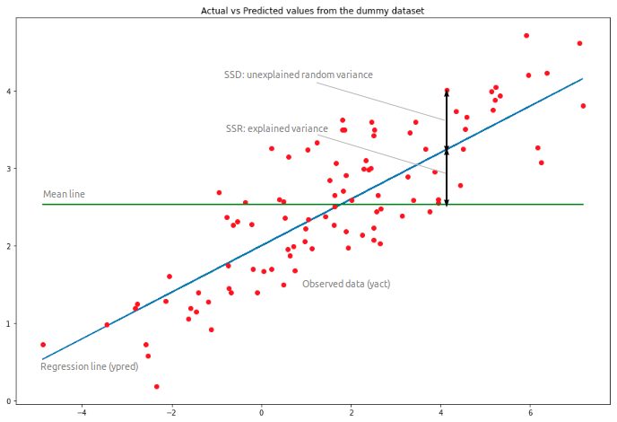
In statistics, linear regression is a linear approach for modelling the relationships between a scalar dependent variable and one (or more) independent variables. The relationships are modelled using linear predictor functions whose unknown model parameters are estimated from the data - known as linear models.

Linear regression has many practical uses which broadly fall into one of the following two categories:

1. Prediction and forecasting which uses linear regression to fit a predictive model to an observed data set of values of the dependent and independent variables using a training data set before using the fitted model to make predictions using a testing data set.

2. Dependent variable variance explanation in which linear regression analysis is used to quantify the relationship between the independent variables and the dependent variable with the goal of identifying which independent variables show a significant linear relationship with the dependent variable.

2   Linear Regression Model

2.1   Formulation

The linear regression model is represented by a linear equation which describes the dependent variable as a linear combination of the independent variables, assigning a coefficient (scale factor) to each input variable with an additional coefficient representing the intercept.

Given a data set ${y_i, x_{i1}, …,x_{ip} }$ consisting of $n$ statistical units, the linear regression model assumes a linear relationship between dependent variable $y$ and the vector of $p$ independent variables. The relationship is modelled through an error variable $\epsilon$ which is an unobserved random variable that adds **noise** to the relationship.

We can write the expression for our linear regression model as:

\[y_i=\beta_0+\beta_1x_{i1}+…+\beta_p x_{ip}+\epsilon_i=\boldsymbol{x}_i^T\boldsymbol{\beta}+\epsilon_i~,\]

where $\beta_0$ is the intercept and $\beta_i$ are our independent variable coefficients.

2.2   Matrix Notation

These $n$ equations (one for each statistical unit) can be written in matrix motation as:

\[\boldsymbol{y}=X\boldsymbol{\beta}+\boldsymbol{\epsilon}~,\]

where:

\[ X = \left(\begin{array}{c} x_1^T \\ x_2^T \\ \vdots \\ x_n^T \end{array}\right) =\left(\begin{array}{ccc} 1 & x_{11} & \cdots & x_{1p} \\ 1 & x_{21} & \cdots & x_{2p} \\ \vdots & \vdots & \ddots & \vdots \\ 1 & x_{n1} & \cdots & x_{np} \end{array}\right) \]

\[\boldsymbol{y}=\begin{pmatrix}y_1\\y_2\\\vdots\\y_n\end{pmatrix},~~\boldsymbol{\beta}=\begin{pmatrix}\beta_0\\ \beta_1\\ \beta_2\\ \vdots\\ \beta_p\end{pmatrix}, ~~ \boldsymbol{\epsilon}\begin{pmatrix}\epsilon_1\\ \epsilon_2\\ \vdots\\ \epsilon_n\end{pmatrix}\]

Here $\boldsymbol{y}$ is the vector of observed values, $\boldsymbol{\beta}$ is the $(p+1)$-dimensional coefficient vector (with intercept $\beta_0$), $X$ is the matrix of $n$-dimensional independent variables $X_j$ (where 1 corresponds $\beta_0$), and $\boldsymbol{\epsilon}$ is the noise vector.

2.3   Assumptions

Standard linear regression models with standard estimation techniques make the following assumptions:

1. Linearity - The mean of the dependent variable is a linear combination of the regression coefficients and the independent variables.

2. Homoscedasticity - The variance of the errors does not depend on the values of the independent variables (this is often not the case).

3. Weak exogeneity - The independent variables can be treated as fixed values rather than random variables (assumed to be error free).

4. Error independence - The errors of the dependent variables are uncorrelated with each other.

5. Lack of perfect multicollinearity - The design matrix $X$ must have full column rank $p$, otherwise a linear relationship exists between two or more predictor variables.

3   Linear Regression & Machine Learning

Learning a linear regression model means estimating the values of the coefficients using our training data set. This can be accomplished in numerous ways but we focus on the following four methods:

3.1   Simple Linear Regression

In simple linear regression we have a single input and therefore we can use statistics to estimate the coefficients. This requires the calculation of statistical properties from the data such as means, standard deviations, correlations and covariance.

3.2   Ordinary Least Squares

When we have multiple inputs we can implement Ordinary Least Squares (OLS) to estimate the values of the coefficients by minimising the sum of squared residuals - i.e. given a line through the data we seek to minimise the value given by calculating the distance from each data point to the regression line, squaring it and summing the squared errors.

This approach treats the data as a matrix and uses linear algebra operations to estimate the optimal values for the coefficients - therefore requires all the data must be available and requires sufficient memory to fit the data and perform matrix operations.

3.3   Gradient Descent

When there are one or more inputs, we can use a process of optimizing the values of the coefficients by iteratively minimizing the error of the model on your training data in a process known as gradient descent.

We start with random values for each coefficient before calculating the sum of the squared errors for each pair of input and output values. A learning rate is used as a scale factor and the coefficients are updated in the direction towards minimising the error. The process is repeated until a minimum sum squared error is achieved or no further improvement is possible.

When implementing this method we select a learning rate (alpha) parameter that determines the size of the improvement step to take on each iteration of the procedure.

3.4 Regularisation

There are extensions of the training of the linear model called regularisation methods which seek to both minimise the sum of the squared error of the model on the training data (using OLS) and reduce the complexity of the model (by reducing the number of non-zero coefficients). Two popular regularisation methods for linear regression include:

1. Lasso Regression - where OLS is modified to also minimise the absolute sum of the coefficients.

2. Ridge Regression - where OLS is modified to also minimise the squared absolute sum of the coefficients.

These methods are effective when there is collinearity in our input values and OLS would overfit the training data.

References

1. Linear Regression for Machine Learning, Machine Learning Algorithms, Jason Brownlee, March 25, 2016.

2. A 101 Guide On The Least Squares Regression Method, Edureka, Zulaikha Lateef, November 25, 2020.